Orbit Correction

This tutorial shows how to correct the orbit.

Prerequisites

The tutorial requires an existing pyAML configuration file which includes configuration of the BPM, correctors and orbit correction.

The example uses the configuration provided by the pyaml-test-lattice package.

import numpy as np
import matplotlib.pyplot as plt
from time import sleep
from pyaml.common.constants import Action
from pyaml_test_lattice import configurations

Load the Accelerator

from pyaml.accelerator import Accelerator
accelerator = Accelerator.load(configurations["pyaml/tango/pyaml-cs-oa/fodo_1gev_6d_pyaml-oa.yaml"])

# Print the string representation of the accelerator
print(accelerator)

Accelerator(facility='Synchrotron SOLEIL', machine='sr', simulators=['design'], controls=['live'])

Control Mode Choice

• accelerator.design — runs pyAT locally, no control system needed. Set wait_time = 0.0.

• accelerator.live — connects to the real machine or virtual twin. Set wait_time to allow readback settling (typically 1.5–2 s).

For live control mode you need a running control system or virtual accelerator. If you want to skip this, run the notebook in design` mode only.

# Use the design mode
SR = accelerator.design

# For live mode
# SR = accelerator.live

wait_time = 0.0 if SR == accelerator.design else 2.0

# Print the string representation of the simulator
print(SR)

Simulator(name='design', lattice='/opt/hostedtoolcache/Python/3.11.16/x64/lib/python3.11/site-packages/pyaml_test_lattice/data/lattice/fodo_1gev_6d.json', mat_key=None, n_elements=193)

Orbit Diagnostics and Correctors

# Get BPMs
bpms = SR.bpms.get("BPM")

# Get correctors
hcorr = SR.magnets.get("HCorr")
vcorr = SR.magnets.get("VCorr")

print(f"BPMs: {len(bpms)}, H correctors: {len(hcorr)}, V correctors: {len(vcorr)}")

BPMs: 16, H correctors: 16, V correctors: 16

Orbit Response Matrix

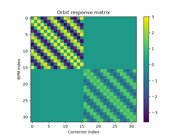
The ORM can be saved in multiple formats. Load it into SR.orbit before correcting.

# Print string representation of the orbit response matrix
print(SR.orm)

OrbitResponseMatrix(name='DEFAULT_ORBIT_RESPONSE_MATRIX', lattice_names='DEFAULT_ORBIT_RESPONSE_MATRIX', peer=Simulator:design, latest_measurement=None, bpms=[BPM(name='BPM_001', lattice_names='BPM_001', peer=Simulator:design, x_pos='AN01-AR/DG-EPOS/BPM.01/x', y_pos='AN01-AR/DG-EPOS/BPM.01/y', x_offset=None, y_offset=None, tilt_name=None), BPM(name='BPM_002', lattice_names='BPM_002', peer=Simulator:design, x_pos='AN02-AR/DG-EPOS/BPM.01/x', y_pos='AN02-AR/DG-EPOS/BPM.01/y', x_offset=None, y_offset=None, tilt_name=None), ... +13 more ..., BPM(name='BPM_016', lattice_names='BPM_016', peer=Simulator:design, x_pos='AN16-AR/DG-EPOS/BPM.01/x', y_pos='AN16-AR/DG-EPOS/BPM.01/y', x_offset=None, y_offset=None, tilt_name=None)], hcorrectors=[HCorrector(name='COR_001.hcorrector', lattice_names='COR_001...

Measure the ORM

SR.orm.measure(sleep_between_step=wait_time)
SR.orm.save("orm.json")
SR.orm.save("orm.yaml", with_type="yaml")

SR.orbit.load("orm.json")
print("ORM measured, saved and loaded.")

ORM measured, saved and loaded.

Visualise the ORM

orm_data = SR.orm.get()
plt.imshow(np.array(orm_data["matrix"]))
plt.colorbar()
plt.title("Orbit response matrix")
plt.xlabel("Corrector index")
plt.ylabel("BPM index")
plt.show()

Dispersion Measurement

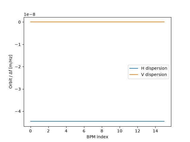
The dispersion can optionally be measured and incorporated into the ORM to enable RF-based orbit correction. This is particularly useful for correcting closed-orbit distortions caused by energy errors.

def disp_callback(action: int, cb_data) -> bool:
    from pyaml.common.constants import Action
    if action == Action.APPLY:
        print("Changing RF frequency")
    elif action == Action.MEASURE:
        print("Reading orbit")
    elif action == Action.RESTORE:
        print("Restoring RF frequency")
    return True

# Measure the dispersion
SR.dispersion.measure(callback=disp_callback)
disp_data = SR.dispersion.get()

# Plot the results
plt.plot(disp_data["frequency_response_x"], label="H dispersion")
plt.plot(disp_data["frequency_response_y"], label="V dispersion")
plt.xlabel("BPM index")
plt.ylabel("Orbit / Δf [m/Hz]")
plt.legend()
plt.show()

Reading orbit
Changing RF frequency
Reading orbit
Changing RF frequency
Reading orbit
Restoring RF frequency
Restoring RF frequency

Introduce Orbit Distortion

Reset correctors to zero, then add small random kicks to simulate a disturbed orbit.

# Reset correctors to zero
hcorr.strengths.set(np.zeros(len(hcorr)))
vcorr.strengths.set(np.zeros(len(vcorr)))
ref_h, ref_v = bpms.positions.get().T
reference = np.concatenate((ref_h, ref_v))

# Add random kicks to simulate a distorted orbit
np.random.seed(1)
std_kick = 1e-6  # rad
hcorr.strengths.set(hcorr.strengths.get() + std_kick * np.random.normal(size=len(hcorr)))
vcorr.strengths.set(vcorr.strengths.get() + std_kick * np.random.normal(size=len(vcorr)))

positions_bc = bpms.positions.get()
std_bc = np.std(positions_bc, axis=0)
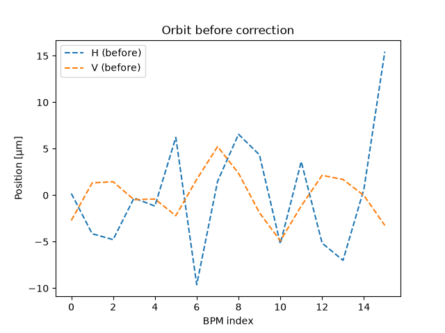
print(f"R.m.s. orbit before correction — H: {1e6 * std_bc[0]:.1f} µm, V: {1e6 * std_bc[1]:.1f} µm")

R.m.s. orbit before correction — H: 6.1 µm, V: 2.5 µm

Orbit Before Correction

plt.figure()
plt.plot(positions_bc[:, 0] * 1e6, label="H (before)", color="C0", ls="--")
plt.plot(positions_bc[:, 1] * 1e6, label="V (before)", color="C1", ls="--")
plt.xlabel("BPM index")
plt.ylabel("Position [µm]")
plt.legend()
plt.title("Orbit before correction")
plt.show()

Correct the Orbit

Standard correction: SR.orbit.correct(reference=reference).

Optional variants (uncomment to use):

• Virtual corrector weight: down-weights correctors that are already at large strengths.

• RF correction: also adjusts the RF frequency to minimise dispersion-driven orbit.

# Standard correction
SR.orbit.correct(reference=reference)

# With virtual corrector weight (ESRF style):
# SR.orbit.set_virtual_weight(1000)
# SR.orbit.correct(reference=reference)

# With RF orbit correction (ESRF style, requires dispersion in ORM):
# SR.orbit.correct(reference=reference, rf=True)

sleep(wait_time)

positions_ac = bpms.positions.get()
std_ac = np.std(positions_ac, axis=0)
print(f"R.m.s. orbit after correction  — H: {1e6 * std_ac[0]:.1f} µm, V: {1e6 * std_ac[1]:.1f} µm")

fig, axes = plt.subplots(3, 1, figsize=(10, 8))

axes[0].plot(positions_ac[:, 0] * 1e6, label="After", color="C0", ls="-")
axes[0].plot(positions_bc[:, 0] * 1e6, label="Before", color="grey", ls="--")

axes[0].set_ylabel("H position [µm]")
axes[0].legend()

axes[1].plot(positions_ac[:, 1] * 1e6, label="After", color="C1", ls="-")
axes[1].plot(positions_bc[:, 1] * 1e6, label="Before", color="grey", ls="--")

axes[1].set_ylabel("V position [µm]")
axes[1].legend()

axes[2].plot(hcorr.strengths.get() * 1e6, label="H correctors")
axes[2].plot(vcorr.strengths.get() * 1e6, label="V correctors")
axes[2].set_ylabel("Strength [µrad]")
axes[2].set_xlabel("Index")
axes[2].legend()

fig.tight_layout()
plt.show()

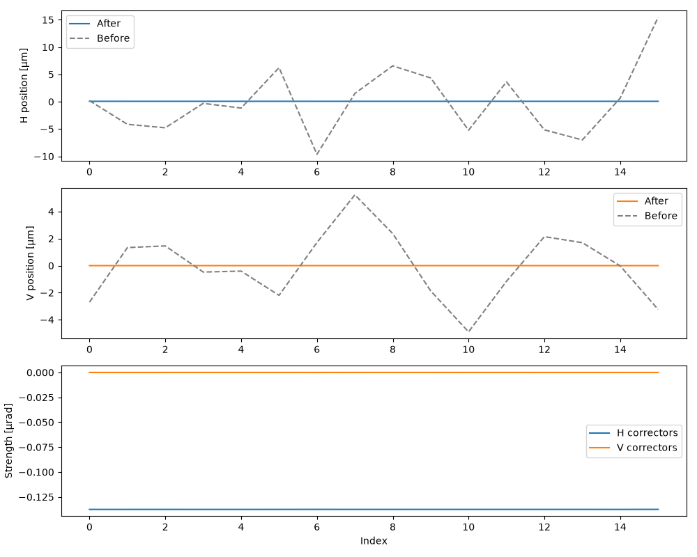
R.m.s. orbit after correction  — H: 0.0 µm, V: 0.0 µm